PID loop tuning using node-red-contrib-pid in node red
This article describes a simple procedure for tuning a loop controlled by the node-red PID node node-red-contrib-pid. The procedure should be satisfactory for tuning reasonably simple processes such as room temperature control, hot water tank temperature control etc. A node-red flow with a simulated process is provided and the procedure works through the tuning of that process. For ease of use the simulation is much faster than most processes the home user will encounter but this makes it easy to try things out and see what the effect is.
Setup
It is assumed that the reader already has a working node-red system. If the pid node is not already installed then do so either from the node-red palette or from the command line using
cd ~/.node-red
npm install node-red-contrib-pid --save
Next import the flow included below. The process is designed to be a little more difficult to control than most that the home user will encounter.
It is highly recommended that the user configures a chart for his process showing the process value and the power output of the PID node. This will be invaluable for understanding how the process is performing.
Tuning: Phase 1. Determine process parameters
The first stage in tuning is to get an estimate of a couple of process parameters. To do this configure the PID loop to on/off control (so it behaves like a thermostat) by setting the Proportional band to 0. The proportional band is in process units, so that is degrees C or whatever your process uses, and determines the range of temperature (or whatever it is) that will change the power output between 0 and 100%, so a setting of 0 means that the power will switch from off to on as the process value crosses the setpoint.
Set the setpoint to one that is appropriate for the process, allowing for the fact that in on/off mode there will be some overshoot above the setpoint (for the simulation use a setpoint of 50). Power the process on and note the time at which the process crosses the setpoint, the time at which the first peak occurs and the value of the process at the peak. Calculate the time taken to go from the setpoint to the first peak and the height of the peak above the setpoint.
For the simulation you should see something like this
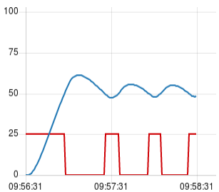
The blue line is the process, cycling round the setpoint of 50 and the red line is the power requested by the PID loop (scaled 0 to 25 so it is visible on the graph) which is switching on and off. For the simulation the time from crossing the setpoint to the first peak is about 12 seconds and the process rises to 61 so the overshoot is 11 units.
Tuning: Phase 2. Initial trial value for Proportional Band
Next we use an initial trial value for the Prob Band of twice the overshoot value above setpoint, so for the simulation set it to 22. We don’t need any integral or derivative effect yet so set the integral to a large time compared to the response of the process. A large integral time equates to minimal integral effect. So for example for a room heating application set the integral to several hours (note that the value entered in the PID node is in seconds). The simulation takes less than a minute to heat up so in this case set it to something like 30 mins (1800 secs). Now repeat the start up operation and see what happens. For the simulation this is simply a matter of re-deploying, for a real process it will be necessary to let it cool down (if it is a heating application) and restart it.
For the simulation we now see:
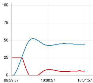
Note that there is a small amount of ‘ringing’ there, but the first peak is much larger than the second (down) peak and the third peak is only just detectable. This is the sort of shape you are looking for in your process at this stage. Note also that it has not settled out on the setpoint but is a little below it. This is because it is the integral terms that pulls it onto the setpoint and because that is set at 1800 it will take around twice that to home in on the setpoint. This will be sorted at the next stage.
If your process is much more stable than the chart above then you can reduce the prop band. I suggest halving it and seeing what happens. If, however, it is showing more ringing than we have here then increase the prop band, possibly doubling it, till you get something similar. The larger the band the less ringing there will be and the smaller it is the more ringing. However it is not that critical, provided there is a bit of overshoot, then it comes down and levels out with minimal ringing then that should be near enough.
Tuning Phase 3: Integral setting
Having got the prop band acceptable the next step is add some integral. Set this to twice the overshoot time that we measured in phase 1, so for the simulation set it to 24 seconds. Restart the process and you should see something like this:
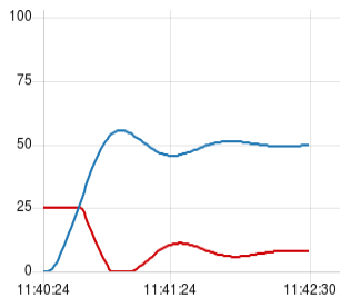
We can see that the integral has had two effects, firstly it has pulled the process right onto the setpoint, but secondly it has increased the ringing. By reducing the integral time we get a more rapid approach to the setpoint, at the expense of reduced stability as is evident by the increased ringing. For a process that is inherently easy to control you may find that there is, in fact, very little, if any overshoot, and it may be that the setting you have at this point is perfectly good enough for your process. However if you do have some overshoot then this is addressed in the next phase.
Tuning: Phase 4. Derivative.
To cut down the overshoot we can now add some derivative. The theoretical ideal value is half of the overshoot time we measured in phase 1, so for the simulation we can set the derivative to 6 seconds, and then this is what we get:
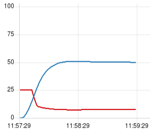
Which is pretty good. A small amount of overshoot and then pulling quickly onto the setpoint.
However, before you get over excited and try that on your process there are some caveats. Derivative works by measuring the rate of rise or fall of the process and cutting the power down if it is approaching the setpoint too fast. This is fine if the process is a clean simulation (as in the example here) but in the real world process signals are noisy (they bump up and down a bit) and in the case of a sensor such as the DS18B20 they have a limited resolution, so even if the process is rising smoothly the value seen by node red will go up in steps (of 0.0625C in the case of the DS18B20). The effect of the noise and process steps is to make the power signal out of the PID node noisy, but it is amplified by the derivative and can cause problems. This is one of the reasons for plotting the power on the chart, so that the noise can be seen. I suggest therefore first trying the derivative as calculated above, but then see what is happening to the power.
If you find that the power is bumping up and down more than about 10 or 15% of full power then you can try using the Derivative Smoothing Factor value that the node provides for just this purpose. Try setting it initially to 3 and see if that reduces the power noise enough, if not then try 5. If it is still too noisy then you have little option other than to reduce the derivative till the noise on the power is ok.
Having got to this point either with the recommended derivative or the maximum your process will cope with then it is possible that the process still overshoots too much for you or rings too much. In that case I suggest doubling the prop band and the integral and try that. The result should be to cut down the overshoot but also to slow down the approach to the setpoint. You can see the effect of this on the simulation by setting the derivative back to zero and doubling prop band and integral to 44 and 48 respectively. This is the result with the simulation:
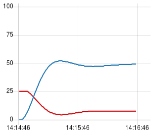
You can see that this is better than the response from phase 3 but is not as good as with the derivative included.
Where now?
The simulation shown here is, of course, an idealised situation and in the real world you may find all sorts of other problems come into play. With room heating for example one of the issues is that it takes so long to stabilise. You may find you only get one or two runs per day which can be a bit tedious. Also factors such as people leaving doors open, the number of people in the room varying (which can easily raise/lower the temperature by 0.5C) and so on. So your experience is unlikely to be as smooth as seen here. An important point is to keep careful notes of what you have done so you can look back and see what you did and what the effect was. If you are using something like influxdb and grafana then it is easy to go back and remind yourself what the chart looked like, but if using more simple graphs such as supplied by the node red dashboard then this is not necessarily possible. In this case I suggest you take regular screenshots so you can look back. Or start using influxdb and grafana of course, which I highly recommend. Once you have it setup and working you will wonder how you survived without it.
Hopefully the above techniques will at least get to a reasonably controlled system.
If you have problems then by all means ask on the node red mailing list.
Here is the example flow:
[
    {
        "id": "b4973237.46ab6",
        "type": "subflow",
        "name": "Process Simulation",
        "info": "",
        "in": [
            {
                "x": 37,
                "y": 103,
                "wires": [
                    {
                        "id": "ec719d4d.0d54f8"
                    }
                ]
            }
        ],
        "out": [
            {
                "x": 728.5,
                "y": 294,
                "wires": [
                    {
                        "id": "ae1a6e5.d4c0d9",
                        "port": 0
                    }
                ]
            }
        ]
    },
    {
        "id": "7fe4b5c3.32e58c",
        "type": "function",
        "z": "b4973237.46ab6",
        "name": "30 sec RC + 20",
        "func": "// Applies a simple RC low pass filter to incoming payload values\nvar tc = 30*1000;       // time constant in milliseconds\n\nvar lastValue = context.get('lastValue');\nif (typeof lastValue == \"undefined\") lastValue = msg.payload;\nvar lastTime = context.get('lastTime') || null;\nvar now = new Date();\nvar currentValue = msg.payload;\nif (lastTime === null) {\n    // first time through\n    newValue = currentValue;\n} else {\n    var dt = now - lastTime;\n    var newValue;\n    \n    if (dt > 0) {\n        var dtotc = dt / tc;\n        newValue = lastValue * (1 - dtotc) + currentValue * dtotc;\n    } else {\n        // no time has elapsed leave output the same as last time\n        newValue = lastValue;\n    }\n}\ncontext.set('lastValue', newValue);\ncontext.set('lastTime', now);\n\nmsg.payload = newValue + 20;\nreturn msg;",
        "outputs": 1,
        "noerr": 0,
        "x": 626.5,
        "y": 207,
        "wires": [
            [
                "ae1a6e5.d4c0d9"
            ]
        ]
    },
    {
        "id": "1bacd004.9753c",
        "type": "inject",
        "z": "b4973237.46ab6",
        "name": "Inject -0.2 at start",
        "topic": "",
        "payload": "-0.2",
        "payloadType": "num",
        "repeat": "",
        "crontab": "",
        "once": true,
        "x": 134.5,
        "y": 30,
        "wires": [
            [
                "ec719d4d.0d54f8"
            ]
        ]
    },
    {
        "id": "999a52c2.f465f",
        "type": "function",
        "z": "b4973237.46ab6",
        "name": "10 sec RC",
        "func": "// Applies a simple RC low pass filter to incoming payload values\nvar tc = 10*1000;       // time constant in milliseconds\n\nvar lastValue = context.get('lastValue');\nif (typeof lastValue == \"undefined\") lastValue = msg.payload;\nvar lastTime = context.get('lastTime') || null;\nvar now = new Date();\nvar currentValue = msg.payload;\nif (lastTime === null) {\n    // first time through\n    newValue = currentValue;\n} else {\n    var dt = now - lastTime;\n    var newValue;\n    \n    if (dt > 0) {\n        var dtotc = dt / tc;\n        newValue = lastValue * (1 - dtotc) + currentValue * dtotc;\n    } else {\n        // no time has elapsed leave output the same as last time\n        newValue = lastValue;\n    }\n}\ncontext.set('lastValue', newValue);\ncontext.set('lastTime', now);\n\nmsg.payload = newValue;\nreturn msg;",
        "outputs": 1,
        "noerr": 0,
        "x": 451,
        "y": 207,
        "wires": [
            [
                "7fe4b5c3.32e58c"
            ]
        ]
    },
    {
        "id": "ec719d4d.0d54f8",
        "type": "delay",
        "z": "b4973237.46ab6",
        "name": "",
        "pauseType": "delay",
        "timeout": "1",
        "timeoutUnits": "seconds",
        "rate": "1",
        "rateUnits": "second",
        "randomFirst": "1",
        "randomLast": "5",
        "randomUnits": "seconds",
        "drop": false,
        "x": 268,
        "y": 104,
        "wires": [
            [
                "ede39236.1961f8"
            ]
        ]
    },
    {
        "id": "a823c9cf.2a6178",
        "type": "function",
        "z": "b4973237.46ab6",
        "name": "2 msg transport delay",
        "func": "// stores messages in a fifo until the specified number have been received, \n// then releases them as new messages are received.\n// during the filling phase the earliest message is passed on each time \n// a message is received, but it is also left in the fifo\nvar fifoMaxLength = 2;\nvar fifo = context.get('fifo') || [];\n// push the new message onto the top of the array, messages are shifted down and\n// drop off the front\nvar length = fifo.push(msg);  // returns new length\nif (length > fifoMaxLength) {\n    newMsg = fifo.shift();\n} else {\n    // not full yet, make a copy of the msg and pass it on\n    var newMsg = JSON.parse(JSON.stringify(fifo[0]));\n}\ncontext.set('fifo', fifo);\nreturn newMsg;",
        "outputs": 1,
        "noerr": 0,
        "x": 258,
        "y": 208,
        "wires": [
            [
                "999a52c2.f465f"
            ]
        ]
    },
    {
        "id": "ae1a6e5.d4c0d9",
        "type": "function",
        "z": "b4973237.46ab6",
        "name": "Clear all except payload",
        "func": "msg2 = {payload: msg.payload};\nreturn msg2;",
        "outputs": 1,
        "noerr": 0,
        "x": 545,
        "y": 293,
        "wires": [
            []
        ]
    },
    {
        "id": "ede39236.1961f8",
        "type": "range",
        "z": "b4973237.46ab6",
        "minin": "0",
        "maxin": "1",
        "minout": "0",
        "maxout": "100",
        "action": "scale",
        "round": false,
        "name": "",
        "x": 87,
        "y": 208,
        "wires": [
            [
                "a823c9cf.2a6178"
            ]
        ]
    },
    {
        "id": "e0cb2a8c.4402a8",
        "type": "PID",
        "z": "f0414dd0.dd514",
        "name": "",
        "setpoint": "50",
        "pb": "0",
        "ti": "0",
        "td": "0",
        "integral_default": "0",
        "smooth_factor": "0",
        "max_interval": 600,
        "enable": "1",
        "disabled_op": "0",
        "x": 362,
        "y": 175,
        "wires": [
            [
                "5ec4239b.34e174",
                "e94f888a.130a88"
            ]
        ]
    },
    {
        "id": "f70949c8.aab988",
        "type": "change",
        "z": "f0414dd0.dd514",
        "name": "",
        "rules": [
            {
                "t": "set",
                "p": "topic",
                "pt": "msg",
                "to": "op",
                "tot": "str"
            }
        ],
        "action": "",
        "property": "",
        "from": "",
        "to": "",
        "reg": false,
        "x": 601.5,
        "y": 250,
        "wires": [
            [
                "9f58a52d.076dd"
            ]
        ]
    },
    {
        "id": "2792f805.066c78",
        "type": "inject",
        "z": "f0414dd0.dd514",
        "name": "Setpoint 30",
        "topic": "setpoint",
        "payload": "30",
        "payloadType": "num",
        "repeat": "",
        "crontab": "",
        "once": false,
        "x": 104,
        "y": 198,
        "wires": [
            [
                "e0cb2a8c.4402a8"
            ]
        ]
    },
    {
        "id": "1bf3ce16.c3ae02",
        "type": "inject",
        "z": "f0414dd0.dd514",
        "name": "Setpoint 80",
        "topic": "setpoint",
        "payload": "80",
        "payloadType": "num",
        "repeat": "",
        "crontab": "",
        "once": false,
        "x": 102.5,
        "y": 247,
        "wires": [
            [
                "e0cb2a8c.4402a8"
            ]
        ]
    },
    {
        "id": "f69bbf05.bdd49",
        "type": "inject",
        "z": "f0414dd0.dd514",
        "name": "enable",
        "topic": "enable",
        "payload": "true",
        "payloadType": "bool",
        "repeat": "",
        "crontab": "",
        "once": false,
        "x": 95,
        "y": 83,
        "wires": [
            [
                "e0cb2a8c.4402a8"
            ]
        ]
    },
    {
        "id": "143523b2.2f165c",
        "type": "inject",
        "z": "f0414dd0.dd514",
        "name": "disable",
        "topic": "enable",
        "payload": "false",
        "payloadType": "bool",
        "repeat": "",
        "crontab": "",
        "once": false,
        "x": 95.5,
        "y": 133,
        "wires": [
            [
                "e0cb2a8c.4402a8"
            ]
        ]
    },
    {
        "id": "5ec4239b.34e174",
        "type": "subflow:b4973237.46ab6",
        "z": "f0414dd0.dd514",
        "x": 365,
        "y": 102,
        "wires": [
            [
                "de738fc5.75e4c8",
                "e0cb2a8c.4402a8"
            ]
        ]
    },
    {
        "id": "de738fc5.75e4c8",
        "type": "change",
        "z": "f0414dd0.dd514",
        "name": "",
        "rules": [
            {
                "t": "set",
                "p": "topic",
                "pt": "msg",
                "to": "pv",
                "tot": "str"
            }
        ],
        "action": "",
        "property": "",
        "from": "",
        "to": "",
        "reg": false,
        "x": 586,
        "y": 101,
        "wires": [
            [
                "9f58a52d.076dd"
            ]
        ]
    },
    {
        "id": "e94f888a.130a88",
        "type": "range",
        "z": "f0414dd0.dd514",
        "minin": "0",
        "maxin": "1",
        "minout": "0",
        "maxout": "25",
        "action": "scale",
        "round": false,
        "name": "Scale power",
        "x": 427,
        "y": 250,
        "wires": [
            [
                "f70949c8.aab988"
            ]
        ]
    },
    {
        "id": "9f58a52d.076dd",
        "type": "ui_chart",
        "z": "f0414dd0.dd514",
        "name": "",
        "group": "c45a83a3.d00908",
        "order": 0,
        "width": "6",
        "height": "6",
        "label": "chart",
        "chartType": "line",
        "legend": "false",
        "xformat": "HH:mm:ss",
        "interpolate": "linear",
        "nodata": "",
        "dot": false,
        "ymin": "0",
        "ymax": "100",
        "removeOlder": "3",
        "removeOlderPoints": "",
        "removeOlderUnit": "60",
        "cutout": 0,
        "useOneColor": false,
        "colors": [
            "#1f77b4",
            "#cf0005",
            "#ff7f0e",
            "#2ca02c",
            "#98df8a",
            "#d62728",
            "#ff9896",
            "#9467bd",
            "#c5b0d5"
        ],
        "useOldStyle": false,
        "x": 791,
        "y": 175,
        "wires": [
            [],
            []
        ]
    },
    {
        "id": "bef0a1f8.2e2cf",
        "type": "inject",
        "z": "f0414dd0.dd514",
        "name": "Clear chart on deploy",
        "topic": "",
        "payload": "{\"data\":[]}",
        "payloadType": "json",
        "repeat": "",
        "crontab": "",
        "once": true,
        "x": 352,
        "y": 318,
        "wires": [
            [
                "9079ffaf.4a096"
            ]
        ]
    },
    {
        "id": "9079ffaf.4a096",
        "type": "change",
        "z": "f0414dd0.dd514",
        "name": "",
        "rules": [
            {
                "t": "move",
                "p": "payload.data",
                "pt": "msg",
                "to": "payload",
                "tot": "msg"
            }
        ],
        "action": "",
        "property": "",
        "from": "",
        "to": "",
        "reg": false,
        "x": 588,
        "y": 318,
        "wires": [
            [
                "9f58a52d.076dd"
            ]
        ]
    },
    {
        "id": "c45a83a3.d00908",
        "type": "ui_group",
        "z": "",
        "name": "PID",
        "tab": "80cd4062.93a5",
        "disp": true,
        "width": "6"
    },
    {
        "id": "80cd4062.93a5",
        "type": "ui_tab",
        "z": "",
        "name": "Home",
        "icon": "dashboard"
    }
]